Know Your Sources (Part 1)
This is part of a series of technical essays documenting the computational analysis that undergirds my dissertation, A Gospel of Health and Salvation. For an overview of the dissertation project, you can read the current project description at jeriwieringa.com. You can access the Jupyter notebooks on Github.
My goals in sharing the notebooks and technical essays are three-fold. First, I hope that they might prove useful to others interested in taking on similar projects. In these notebooks I describe and model how to approach a large corpus of sources in the production of historical scholarship.
Second, I am sharing them in hopes that “given enough eyeballs, all bugs are shallow.” If you encounter any bugs, if you see an alternative way to solve a problem, or if the code does not achieve the goals I have set out for it, please let me know!
Third, these notebooks make an argument for methodological transparency and for the discussion of methods as part of the scholarly argument of digital history. Often the technical work in digital history is done behind the scenes, with publications favoring the final research products, usually in article form with interesting visualizations. While there is a growing culture in digital history of releasing source code, there is little discussion of how that code was developed, why solutions were chosen, and what those solutions enable and prevent. In these notebooks I seek to engage that middle space between code and the final analysis - documenting the computational problem solving that I’ve done as part of the analysis. As these essays attest, each step in the processing of the corpus requires the researcher to make a myriad of distinctions about the worlds they seek to model, distinctions that shape the outcomes of the computational analysis and are part of the historical argument of the work.
Now that we have a collection of texts selected and downloaded, and have extracted the text, we need to spend some time identifying what the corpus contains, both in terms of coverage and quality. As I describe in the project overview, I will be using these texts to make arguments about the development of the community’s discourses around health and salvation. While the corpus makes that analysis possible, it also sets the limits of what we can claim from text analysis alone. Without an understanding of what those limits are, we run the risk of claiming more than the sources can sustain, and in doing so, minimizing the very complexities that historical research seeks to reveal.
"""My usual practice for gathering the filenames is to read
them in from a directory. So that this code can be run locally
without the full corpus downloaded, I exported the list
of filenames to an index file for use in this notebook.
"""
with open("data/2017-05-05-corpus-index.txt", "r") as f:
    corpus = f.read().splitlines()
len(corpus)
197943
To create an overview of the corpus, I will use the document filenames along with some descriptive metadata that I created.
Filenames are an often underestimated feature of digital files, but one that can be used to great effect. For my corpus, the team that digitized the periodicals did an excellent job of providing the files with descriptive names. Overall, the files conform to the following pattern:
PrefixYYYYMMDD-V00-00.pdf
I discovered a few files that deviated from the pattern, but renamed those so that the pattern held throughout the corpus. When splitting the PDF documents into pages, I preserved the structure, adding -page0.txt to the end.
The advantage of this format is that the filenames contain the metadata I need to place each file within its context. By isolating the different sections of the filename, I can quickly place any file with reference to the periodical title and the publication date.
import pandas as pd
import re
def extract_pub_info(doc_list):
    """Use regex to extract metadata from filename.

    Note:
        Assumes that the filename is formatted as::

            `PrefixYYYYMMDD-V00-00.pdf`

    Args:
        doc_list (list): List of the filenames in the corpus.
    Returns:
        dict: Dictionary with the year and title abbreviation for each filename.
    """

    corpus_info = {}

    for doc_id in doc_list:

        # Split the ID into three parts on the '-'
        split_doc_id = doc_id.split('-')

        # Get the prefix by matching the first set of letters
        # in the first part of the filename.
        title = re.match("[A-Za-z]+", split_doc_id[0])
        # Get the dates by grabbing all of the number elements
        # in the first part of the filename.
        dates = re.search(r'[0-9]+', split_doc_id[0])
        # The first four numbers is the publication year.
        year = dates.group()[:4]

        # Update the dictionary with the title and year
        # for the filename.
        corpus_info[doc_id] = {'title': title.group(), 'year': year}

    return corpus_info
corpus_info = extract_pub_info(corpus)
One of the most useful libraries in Python for working with data is Pandas. With Pandas, Python users gain much of the functionality that our colleagues who work with R have long celebrated as the benefits of that domain-specific language.
By transforming our corpus_info dictionary into a dataframe, we can quickly filter and tabulate a number of different statistics on our corpus.
df = pd.DataFrame.from_dict(corpus_info, orient='index')
df.index.name = 'docs'
df = df.reset_index()
You can preview the initial dataframe by uncommenting the cell below.
# df
df = df.groupby(["title", "year"], as_index=False).docs.count()
df
| title | year | docs | |
|---|---|---|---|
| 0 | ADV | 1898 | 26 |
| 1 | ADV | 1899 | 674 |
| 2 | ADV | 1900 | 463 |
| 3 | ADV | 1901 | 389 |
| 4 | ADV | 1902 | 440 |
| 5 | ADV | 1903 | 428 |
| 6 | ADV | 1904 | 202 |
| 7 | ADV | 1905 | 20 |
| 8 | ARAI | 1909 | 64 |
| 9 | ARAI | 1919 | 32 |
| 10 | AmSn | 1886 | 96 |
| 11 | AmSn | 1887 | 96 |
| 12 | AmSn | 1888 | 105 |
| 13 | AmSn | 1889 | 386 |
| 14 | AmSn | 1890 | 403 |
| 15 | AmSn | 1891 | 398 |
| 16 | AmSn | 1892 | 401 |
| 17 | AmSn | 1893 | 402 |
| 18 | AmSn | 1894 | 402 |
| 19 | AmSn | 1895 | 400 |
| 20 | AmSn | 1896 | 408 |
| 21 | AmSn | 1897 | 800 |
| 22 | AmSn | 1898 | 804 |
| 23 | AmSn | 1899 | 801 |
| 24 | AmSn | 1900 | 800 |
| 25 | CE | 1909 | 104 |
| 26 | CE | 1910 | 312 |
| 27 | CE | 1911 | 312 |
| 28 | CE | 1912 | 306 |
| 29 | CE | 1913 | 420 |
| ... | ... | ... | ... |
| 465 | YI | 1885 | 192 |
| 466 | YI | 1886 | 220 |
| 467 | YI | 1887 | 244 |
| 468 | YI | 1888 | 104 |
| 469 | YI | 1889 | 208 |
| 470 | YI | 1890 | 208 |
| 471 | YI | 1895 | 416 |
| 472 | YI | 1898 | 28 |
| 473 | YI | 1899 | 408 |
| 474 | YI | 1900 | 408 |
| 475 | YI | 1901 | 408 |
| 476 | YI | 1902 | 408 |
| 477 | YI | 1903 | 408 |
| 478 | YI | 1904 | 288 |
| 479 | YI | 1905 | 408 |
| 480 | YI | 1906 | 408 |
| 481 | YI | 1907 | 432 |
| 482 | YI | 1908 | 832 |
| 483 | YI | 1909 | 844 |
| 484 | YI | 1910 | 850 |
| 485 | YI | 1911 | 852 |
| 486 | YI | 1912 | 868 |
| 487 | YI | 1913 | 848 |
| 488 | YI | 1914 | 852 |
| 489 | YI | 1915 | 852 |
| 490 | YI | 1916 | 852 |
| 491 | YI | 1917 | 840 |
| 492 | YI | 1918 | 850 |
| 493 | YI | 1919 | 856 |
| 494 | YI | 1920 | 45 |
495 rows × 3 columns
Nearly 500 rows of data is too large to have a good sense of the coverage of the corpus from reading the data table, so it is necessary to create some visualizations of the records. For a quick prototyping tool, I am using the Bokeh library.
from bokeh.charts import Bar, show
from bokeh.charts import defaults
from bokeh.io import output_notebook
from bokeh.palettes import viridis
output_notebook()
defaults.width = 900
defaults.height = 950
In this first graph, I am showing the total number of pages per title, per year in the corpus.
p = Bar(df,
        'year',
        values='docs',
        agg='sum',
        stack='title',
        palette= viridis(30),
        title="Pages per Title per Year")
show(p)
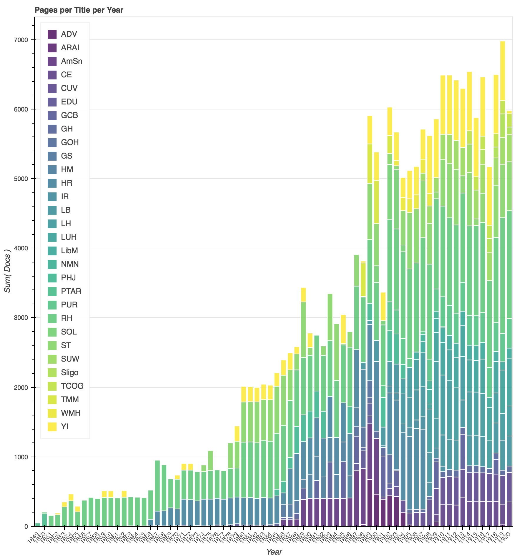
This graph of the corpus reflects the historical development of the publication efforts denomination. Starting with a single publication in 1849, the publishing efforts of the denomination expand in the 1860s as they launch their health reform efforts, expand again in the 1880s as they start a publishing house in California and address concerns about Sunday observance laws, and again at the turn of the century as the denomination reorganizes and regional publications expand. The chart also reveals some holes in the corpus. The Youth’s Instructor (shown here in yellow) in one of the oldest continuous denominational publications, but the pages available for the years from 1850 - 1899 are inconsistent.
In interpreting the results of mining these texts, it will be important to factor in the relative difference in size and diversity of publication venues between the early years of the denomination and the later years of this study.
by_title = df.groupby(["title"], as_index=False).docs.sum()
p = Bar(df,
        'title',
        values='docs',
        color='title',
        palette=viridis(30),
        title="Total Pages by Title"
       )
show(p)
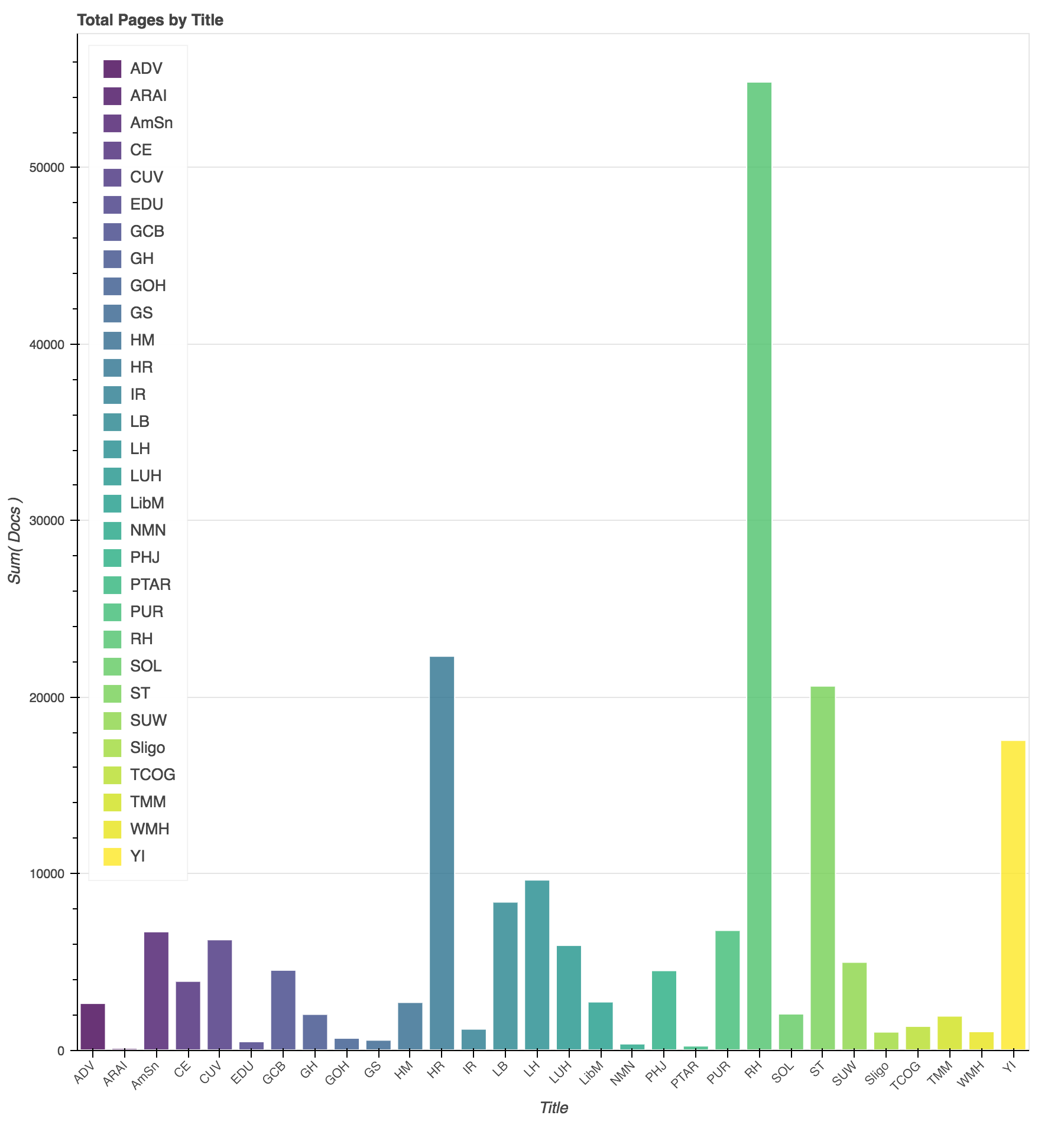
Another way to view the coverage of the corpus is by total pages per periodical title. The Advent Review and Sabbath Herald dominates the corpus in number of pages, with The Health Reformer, Signs of the Times, and the Youth’s Instructor, making up the next major percentage of the corpus. In terms of scale, these publications will have (and had) a prominent role in shaping the discourse of the SDA community. At the same time, it will be informative to look to the smaller publications to see if we can surface alternative and dissonant ideas.
topic_metadata = pd.read_csv('data/2017-05-05-periodical-topics.csv')
topic_metadata
| periodicalTitle | title | startYear | endYear | initialPubLocation | topic | |
|---|---|---|---|---|---|---|
| 0 | Training School Advocate | ADV | 1898 | 1905 | Battle Creek, MI | Education |
| 1 | American Sentinel | AmSn | 1886 | 1900 | Oakland, CA | Religious Liberty |
| 2 | Advent Review and Sabbath Herald | ARAI | 1909 | 1919 | Washington, D.C. | Denominational |
| 3 | Christian Education | CE | 1909 | 1920 | Washington, D.C. | Education |
| 4 | Welcome Visitor (Columbia Union Visitor) | CUV | 1901 | 1920 | Academia, OH | Regional |
| 5 | Christian Educator | EDU | 1897 | 1899 | Battle Creek, MI | Education |
| 6 | General Conference Bulletin | GCB | 1863 | 1918 | Battle Creek, MI | Denominational |
| 7 | Gospel Herald | GH | 1898 | 1920 | Yazoo City, MS | Regional |
| 8 | Gospel of Health | GOH | 1897 | 1899 | Battle Creek, MI | Health |
| 9 | Gospel Sickle | GS | 1886 | 1888 | Battle Creek, MI | Missions |
| 10 | Home Missionary | HM | 1889 | 1897 | Battle Creek, MI | Missions |
| 11 | Health Reformer | HR | 1866 | 1907 | Battle Creek, MI | Health |
| 12 | Indiana Reporter | IR | 1901 | 1910 | Indianapolis, IN | Regional |
| 13 | Life Boat | LB | 1898 | 1920 | Chicago, IL | Missions |
| 14 | Life and Health | LH | 1904 | 1920 | Washington, D.C. | Health |
| 15 | Liberty | LibM | 1906 | 1920 | Washington, D.C. | Religious Liberty |
| 16 | Lake Union Herald | LUH | 1908 | 1920 | Berrien Springs, MI | Regional |
| 17 | North Michigan News Sheet | NMN | 1907 | 1910 | Petoskey, MI | Regional |
| 18 | Pacific Health Journal and Temperance Advocate | PHJ | 1885 | 1904 | Oakland, CA | Health |
| 19 | Present Truth (Advent Review) | PTAR | 1849 | 1850 | Middletown, CT | Denominational |
| 20 | Pacific Union Recorder | PUR | 1901 | 1920 | Oakland, CA | Regional |
| 21 | Review and Herald | RH | 1850 | 1920 | Paris, ME | Denominational |
| 22 | Sligonian | Sligo | 1916 | 1920 | Washington, D.C. | Regional |
| 23 | Sentinel of Liberty | SOL | 1900 | 1904 | Chicago, IL | Religious Liberty |
| 24 | Signs of the Times | ST | 1874 | 1920 | Oakland, CA | Denominational |
| 25 | Report of Progress, Southern Union Conference | SUW | 1907 | 1920 | Nashville, TN | Regional |
| 26 | Church Officer's Gazette | TCOG | 1914 | 1920 | Washington, D.C. | Denominational |
| 27 | The Missionary Magazine | TMM | 1898 | 1902 | Philadelphia, PA | Missions |
| 28 | West Michigan Herald | WMH | 1903 | 1908 | Grand Rapids, MI | Regional |
| 29 | Youth's Instructor | YI | 1852 | 1920 | Rochester, NY | Denominational |
We can generate another view by adding some external metadata for the titles. The “topics” listed here are ones I assigned when skimming the different titles. “Denominational” refers to centrally produced publications, covering a wide array of topics. “Education” refers to periodicals focused on education. “Health” to publications focused on health. “Missions” titles are focused on outreach and evangelism focused publications and “Religious Liberty” on governmental concerns over Sabbath laws. Finally, “Regional” refers to periodicals produced by local union conferences, which like the denominational titles cover a wide range of topics.
by_topic = pd.merge(topic_metadata, df, on='title')
p = Bar(by_topic,
        'year',
        values='docs',
        agg='sum',
        stack='topic',
        palette= viridis(6),
        title="Pages per Topic per Year")
show(p)

Here we can see the diversification of periodical subjects over time, especially around the turn of the century.
p = Bar(by_topic,
        'topic',
        values='docs',
        agg='sum',
        stack='title',
        palette= viridis(30),
        title="Pages per Topic per Year")
p.left[0].formatter.use_scientific = False
p.legend.location = "top_right"
show(p)
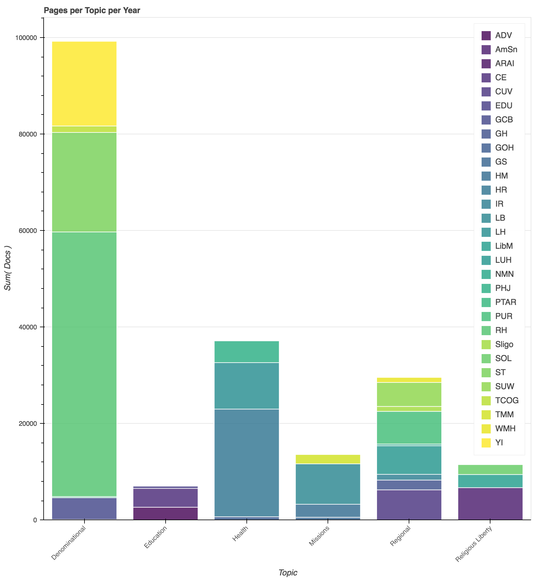
Grouping by category allows us to see that our corpus is dominated by the denominational, health, and regionally focused publications. These topics match with our research concerns, increasing our confidence that we will have enough information to determine meaningful patterns about those topics. But, due to the focus of the corpus, we should proceed cautiously before making any claims about the relative importance of those topics within the community.
Now that we have a sense of the temporal and topical coverage of our corpus, we will next turn our attention to evaluating the quality of the data that we have gathered from the scanned PDF files.
You can run this code locally using the Jupyter notebook available via Github.
Enjoy Reading This Article?
Here are some more articles you might like to read next: